Getting started with Power BI: A beginners guide / tutorial

Power BI is a powerful business analytics tool developed by Microsoft that enables users to visualize data and share insights across the organization, or even embed them in an app or website. It can connect to a broad range of data sources, from Excel spreadsheets to cloud-based and on-premise SQL Server databases, and more. Power BI offers a comprehensive suite of analytics tools that can generate real-time interactive dashboards, produce in-depth reports, and create compelling data visualizations. By using Power BI, businesses can transform raw data into meaningful insights effortlessly, enabling them to make informed decisions. The ability to provide actionable intelligence on key business metrics can lead to improved productivity, better customer service, and a competitive edge in the marketplace.

To help you get started, I’ve put together this simple sales focused tutorial.

Prerequisites

Before you start, you will need:

1) Power BI Desktop to be installed: https://powerbi.microsoft.com/en-gb/downloads/

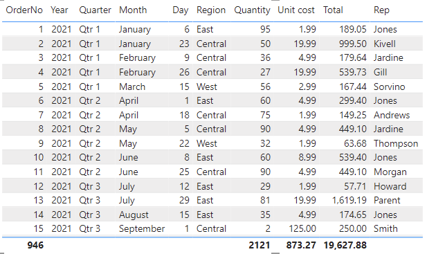
2) Create an excel spreadsheet called ‘PowerBI_SampleData.xlsx’, with the below table of data, and rename the sheet as ‘SalesOrders’:

OrderNo	Order date	Region	Rep	Item	Quantity	Unit cost	Total
1	06/01/2021	East	Jones	Pencil	95	1.99	189.05
2	23/01/2021	Central	Kivell	Binder	50	19.99	999.50
3	09/02/2021	Central	Jardine	Pencil	36	4.99	179.64
4	26/02/2021	Central	Gill	Pen	27	19.99	539.73
5	15/03/2021	West	Sorvino	Pencil	56	2.99	167.44
6	01/04/2021	East	Jones	Binder	60	4.99	299.40
7	18/04/2021	Central	Andrews	Pencil	75	1.99	149.25
8	05/05/2021	Central	Jardine	Pencil	90	4.99	449.10
9	22/05/2021	West	Thompson	Pencil	32	1.99	63.68
10	08/06/2021	East	Jones	Binder	60	8.99	539.40
11	25/06/2021	Central	Morgan	Pencil	90	4.99	449.10
12	12/07/2021	East	Howard	Binder	29	1.99	57.71
13	29/07/2021	East	Parent	Binder	81	19.99	1,619.19
14	15/08/2021	East	Jones	Pencil	35	4.99	174.65
15	01/09/2021	Central	Smith	Desk	2	125.00	250.00
16	18/09/2021	East	Jones	Pen Set	16	15.99	255.84
17	05/10/2021	Central	Morgan	Binder	28	8.99	251.72
18	22/10/2021	East	Jones	Pen	64	8.99	575.36
19	08/11/2021	East	Parent	Pen	15	19.99	299.85
20	25/11/2021	Central	Kivell	Pen Set	96	4.99	479.04
21	12/12/2021	Central	Smith	Pencil	67	1.29	86.43
22	29/12/2021	East	Parent	Pen Set	74	15.99	1,183.26
23	15/01/2022	Central	Gill	Binder	46	8.99	413.54
24	01/02/2022	Central	Smith	Binder	87	15.00	1,305.00
25	07/03/2022	East	Jones	Binder	4	4.99	19.96
26	07/03/2022	West	Sorvino	Binder	7	19.99	139.93
27	07/03/2022	Central	Jardine	Pen Set	50	4.99	249.50
28	10/04/2022	Central	Andrews	Pencil	66	1.99	131.34
29	27/04/2022	East	Howard	Pen	96	4.99	479.04
30	14/05/2022	Central	Gill	Pencil	53	1.29	68.37
31	14/05/2022	Central	Gill	Binder	80	8.99	719.20
32	14/05/2022	Central	Kivell	Desk	5	125.00	625.00
33	04/07/2022	East	Jones	Pen Set	62	4.99	309.38
34	21/07/2022	Central	Morgan	Pen Set	55	12.49	686.95
35	21/07/2022	Central	Kivell	Pen Set	42	23.95	1,005.90
36	21/07/2022	West	Sorvino	Desk	3	275.00	825.00
37	10/09/2022	Central	Gill	Pencil	7	1.29	9.03
38	10/09/2022	West	Sorvino	Pen	76	1.99	151.24
39	10/09/2022	West	Thompson	Binder	57	19.99	1,139.43
40	31/10/2022	Central	Andrews	Pencil	14	1.29	18.06
41	31/10/2022	Central	Jardine	Binder	11	4.99	54.89
42	04/12/2022	Central	Jardine	Binder	94	19.99	1,879.06
43	21/12/2022	Central	Andrews	Binder	28	4.99	139.72

Save your spreadsheet, and make sure Excel is closed.

Creating a Power BI report

To create your first report, using the above spreadsheet as the data source, follow the below steps:

1) Open the ‘Power BI Desktop’ application

2) Select ‘Get data’

3) Select the ‘Excel’ as the data type, click ‘Connect’ and select your excel file. See the prerequisites for reference to sample data for this guide

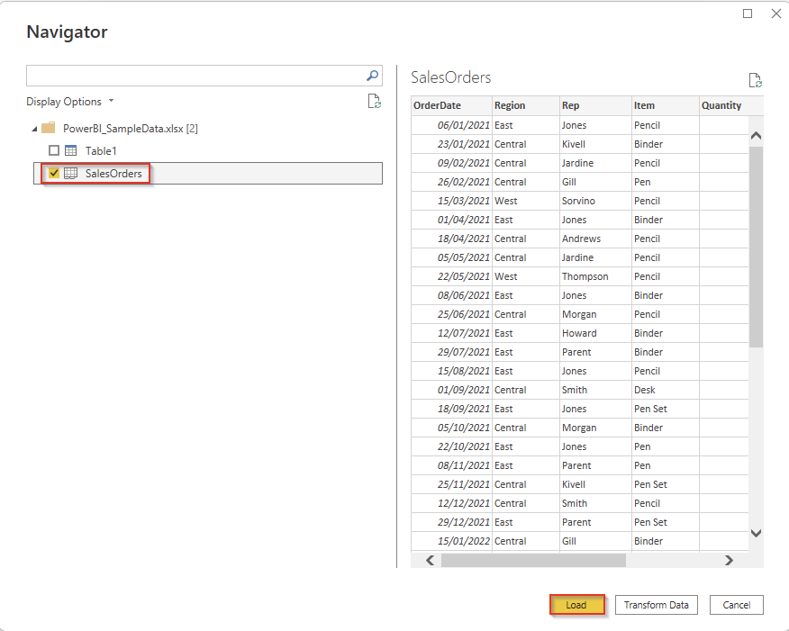
4) You will now see a list of worksheets and tables (if you use them). I’d recommend using worksheets over tables, and in this example it the worksheet we want is called ‘SalesOrders’. Select it, and click ‘Load’

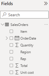
5) You will no see ‘SalesOrder’ under the fields section to the right of the screen. Expand it by selecting the > symbol

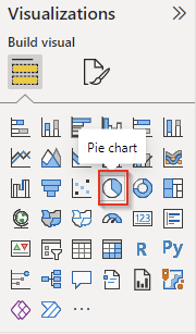
6) From the visualisation section, select ‘pie chart’, and you will then see a blank pie chart appear on the screen

7) For this pie chart, we’ll display orders by region. To do this, drag ‘Region’ from the fields area to the ‘Legend’ box in the visualisation area, and then drag ‘OrderNo’ to the values area

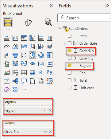
(tip: you must have the blank pie chart selected to see this option)

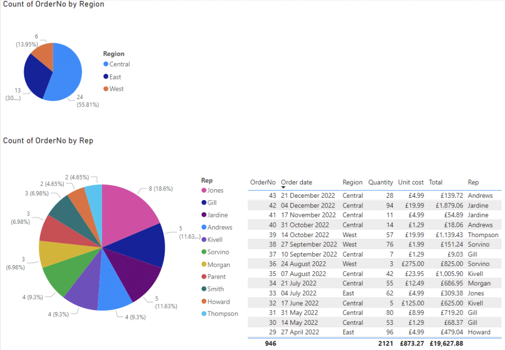
8) You should now see a pie chart that looks like this:

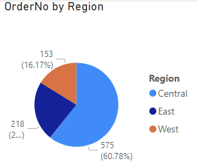
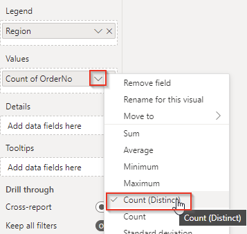
However, this is wrong, as the default action is to add up the values from the ‘OrderNo’ field, where we just want to count how many there are. To change this, make sure your pie chart is selected, select the down arrow on ‘OrderNo’ and select count (distinct).

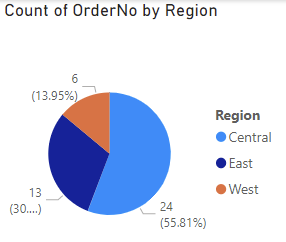
This then changes the pie chart to look like this:

9) Repeat the same steps to create another new pie chart, but replace ‘Region’ with ‘Rep’ and you should see a pie chart that looks like this

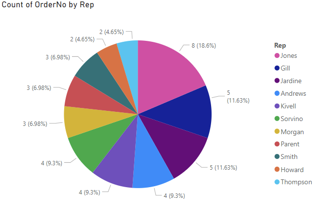
I have resized my chart to show the ‘Rep’ names, you can do the same

(tip: unselect any tables or charts by clicking a blank area outside of the chart/page before select your visualisation type (e.g. pie chart), as otherwise it will change the selected chart)

10) These charts are interactive, so when you click on a rep’s name, the orders by region will change to help you visualise how many sales that rep made in each region

11) You can also change the titles and various other settings for each chart by selecting a chart, and clicking the ‘Format your visual’ icon at the top of the visualisation area

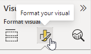
A favourite of mine is to change the colours, location of legend and detail labels, but you will discover what you like as you work through the options

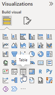
12) We’ll now add a data table to the report by selecting the ‘Table’ visual in the visualisations area

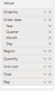
13) To add the data, just drag each column into the values area, as I have below:

This then results in a table like this:

14) You’ll notice the dates look strange, to fix that there are a number of different approaches, but the easiest is to right click on the ‘Order date’ column under and select ‘Create hierarchy’

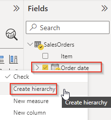
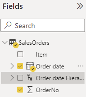
A new column will then appear in for you to use

15) Now the date is fixed, select your table again, remove the order date field/s and add the new one in its place. It should then look like this:

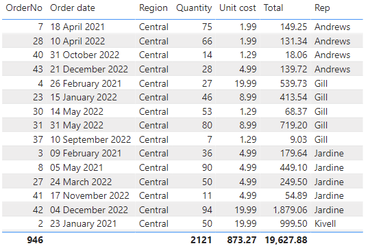
(tip: you can drag the items to change the column order)

16) You can change order of the data on each visual by selecting it, then the three dots, followed b

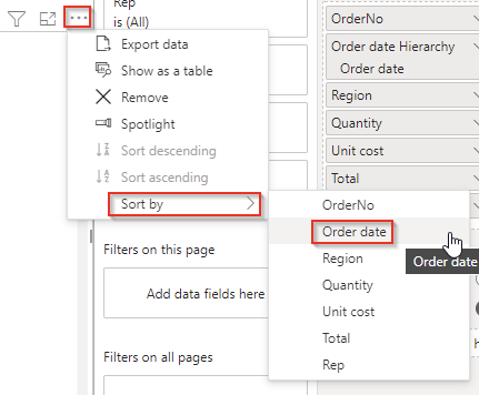
When you have selected a field to order by, you can also select if it should be ascending or descending

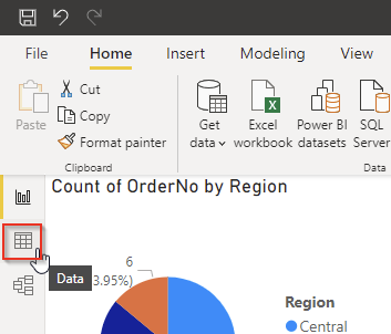
17) The table now looks good, but if you’d like to add a currency symbol to the unit cost and total columns, you need to select ‘Data’ icon to the top left of the screen

Select the ‘Unit cost’ column and change the Format to currency

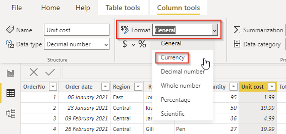
Then set the symbol as you’d like it by selecting the small down arrow next to the currency/dollar button

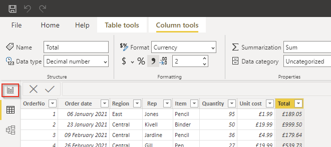
Do the same for the ‘Total’ column

18) You can now return to your report by selecting the ‘Report’ icon toward the top left of the screen

19) You should now have something that looks like the below, and as mentioned above, it’s all interactive

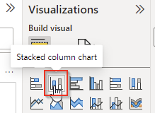
20) Now lets visualise the sales by month, by adding a new bar chart. There are many types, but I’ll add a stacked column chart, to allow us to also see how much was for each region

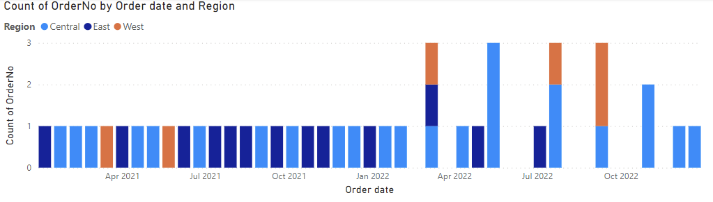
21) Drag the new data column, which we created earlier, to the ‘Axis’ field, ‘Region’ to the ‘Legend field and ‘OrderNo’ to the ‘Values’ field. Don’t forget to change ‘OrderNo’ to count (distinct again)

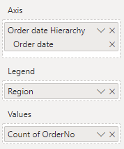
You should then see a graph like this:

22) If you haven’t already, save your Power BI report, and experiment with the visualisation formatting, and add additional pages too, if you want